Beef Muscle Tenderness Ranking Case Brooks Shear Force

Article Card

/ajax/scifeed/subscribe

Open up Access Commodity

Beef Tenderness Prediction by a Combination of Statistical Methods: Chemometrics and Supervised Learning to Manage Integrative Farm-To-Meat Continuum Data

¹

UMR Herbivores, VetAgro Sup, Université Clermont Auvergne, INRA, F-63122 Saint-Genès-Champanelle, France

²

URSE, Ecole Supérieure d'Agriculture (ESA), Université Bretagne Loire, 55 Rue Rabelais, BP 30748, 49007 Angers, CEDEX, French republic

^*

Authors to whom correspondence should exist addressed.

Received: 3 July 2019 / Revised: 15 July 2019 / Accepted: 19 July 2019 / Published: 22 July 2019

Abstract

This trial aimed to integrate metadata that spread over farm-to-fork continuum of 110 Protected Designation of Origin (PDO)Maine-Anjou cows and combine ii statistical approaches that are chemometrics and supervised learning; to identify the potential predictors of beef tenderness analyzed using the instrumental Warner-Bratzler Shear force (WBSF). Accordingly, 60 variables including WBSF and belonging to 4 levels of the continuum that are subcontract-slaughterhouse-musculus-meat were analyzed by Partial Least Squares (PLS) and three decision tree methods (C&RT: classification and regression tree; QUEST: quick, unbiased, efficient regression tree and CHAID: Chi-squared Automatic Interaction Detection) to select the driving factors of beef tenderness and suggest predictive decision tools. The old method retained 24 variables from 59 to explain 75% of WBSF. Among the 24 variables, six were from farm level, four from shambles level, 11 were from musculus level which are by and large protein biomarkers, and three were from meat level. The decision trees applied on the variables retained by the PLS model, allowed identifying three WBSF classes (Tender (WBSF ≤ 40 N/cm²), Medium (xl Due north/cm² < WBSF < 45 Due north/cm²), and Tough (WBSF ≥ 45 N/cm^two)) using CHAID as the best decision tree method. The resultant model yielded an overall predictive accuracy of 69.4% by v splitting variables (full collagen, µ-calpain, fiber area, age of weaning and ultimate pH). Therefore, two determination model rules allow achieving tender meat on PDO Maine-Anjou cows: (i) IF (total collagen < 3.6 μg OH-proline/mg) AND (µ-calpain ≥ 169 capricious units (AU)) AND (ultimate pH < five.55) THEN meat was very tender (mean WBSF values = 36.2 N/cmⁱⁱ, n = 12); or (2) IF (total collagen < 3.six μg OH-proline/mg) AND (µ-calpain < 169 AU) AND (age of weaning < 7.75 months) AND (fiber expanse < 3100 µmⁱⁱ) Then meat was tender (mean WBSF values = 39.four N/cm², north = xxx).

1. Introduction

Amid the eating qualities of meat, tenderness is often reported as ane of the master drivers of beefiness palatability that dictates the overall liking of cooked meat or to brand (re)purchasing decision [one,2,3]. Even so, it has been reviewed that for consumer confidence, at that place is need to guarantee consistent and loftier eating quality of meat [4]. From the large literature, there is a consensus that this is a challenging chore to achieve consistent eating quality equally meat is biochemically dynamic and susceptible to variation. Indeed, variations in beefiness tenderness stems from a wide range of factors which are intrinsic and extrinsic and measurable from the farm-to-fork continuum levels [5,6,7,eight]. The modern beef industry seeks new strategies using the whole or function of these factors to develop management and predictive tools. These tools would provide products of consequent quality that meet consumer expectations, paying specific attending to sensory traits. Accordingly, nosotros recently proposed a holistic arroyo that considers 4 levels of the farm-to-fork alive flow of the animals (farm level: rearing factors and beast characteristics, slaughter-house level: carcass characteristics, musculus level: muscle characteristics and protein biomarkers, meat level: meat quality traits) to sufficiently characterize the driving factors in relation to dissimilar desirable qualities of meat, namely tenderness [eight,9].

Therefore, we intend to use metadata that spread over this continuum, to identify how carcass and beef qualities can be jointly managed using rearing practices applied during the whole life of the animals or by a combination of proxies that vest to the other levels of the continuum [8]. To attain this challenging objective, we proposed to implement various statistical strategies to analyze this metadata past defining 3 main purposes: (i) utilize/develop appropriate statistical tools to relate accurately the different elements of the continuum; (two) determine the most appropriate methods of rearing practices to meet the expectations of the slaughterers; and (3) provide breeders/slaughterers with determination tools (predictive) for joint management of carcass and meat quality potential [10]. Hence, partial least squares regression (PLS) and decision copse were applied in this work to achieve the fixed objectives on PDO Maine-Anjou choose cows. Overall, the combined statistical techniques used in this trial showed the possibility to propose recommendations that would help brand decisions nigh how joint direction of the qualities of carcasses and their produced beef will aid accomplish the targeted market specifications.

2. Materials and Methods

2.ane. Experimental Blueprint and Animate being Characteristics and Rearing Factors

In this trial, we used the data of the same 110 PDO Maine-Anjou cows from previous experimental designs that are described in details by Gagaoua et al. [11] and Couvreur et al. [12]. The investigated cows are from a cooperative of livestock farmers located in the department of Maine-et-Loire, France. All the animals were nerveless and slaughtered following the same protocol and in the aforementioned commercial shambles (Elivia, King of beasts d'Angers, French republic). This collaboration immune united states collecting data on animals such the feeding regimen during the whole life of the animal besides as the day before slaughter, conditions of transport to the shambles and duration, conditions of resting flow after inflow at the abattoir, conditions of resting with free admission to water but nutrient deprived, stunning procedure, as well the weather condition of chilling and storing of the carcasses.

The rearing practices of each animal were obtained by a survey carried out by directly interviewing farmers and described in detail by Couvreur et al. [12]. The survey included 16 quantitative and qualitative questions (Table 1) subdivided into 2 categories:

(i)

Questions related to the finishing period: role of hay, haylage and/or grass in the finishing diet (% w/w); daily and global amount of concentrate (kg); fattening duration (days); concrete activeness (% days out)

(ii)

Questions related to animal characteristics: animals with beefiness or dairy-power; birth month/season; nascence weight (kg); historic period at weaning (month); duration of the period between the concluding weaning and the starting time of the finishing menstruation (days); age of kickoff calving; number of calving; suckling value (0–10) and age at slaughter.

2.ii. Slaughtering, Carcass Characteristics and Muscle Sampling

All the cows were slaughtered using convict bolt pistol prior to exsanguination. They were dressed following the standard commercial practices in compliance with the French welfare and EU regulations (Council Regulation (EC) No. 1099/2009). The carcasses were not electrically stimulated. We chilled the carcasses during 24 h p-m (post mortem) at 2–iii °C. Later slaughter, the carcasses were characterized and graded using the European beef grading system (CE 1249/2008). A full of 8 carcass characteristics (Table two) were recorded: the carcass weight (kg), conformation score (ane–15 calibration), weight of the fifth ribeye, musculus carcass weight (g) of the 5th rib, fat carcass weight (g) of the 5th rib, fat-to-musculus ratio in the 5th rib (% due west/due west), color score of the carcass (1–5 scale) and tenderness score of the carcass (one–5 scale).

The Longissimus thoracis (LT, mixed fast oxido-glycolytic) muscle samples were removed from the correct-hand side of each animate being carcass 24 h p-m from as detailed in Gagaoua et al. [xi]. Briefly, from the four parts that were taken, one was frozen in liquid nitrogen and kept at −fourscore °C until analyzed for musculus biochemistry past the quantification of fiber area, the percentages of myosin heavy chains isoforms (MyHC), the activities of metabolic enzymes describing both the glycolytic and oxidative pathways, biomarkers of beefiness tenderness quantified by the immunobased Dot-Blot technique. The second part was cut into pieces of 1–2 cm cross-department, vacuum packed and stored at −20 °C until analyzed for intramuscular fat content and intramuscular connective tissue. The 3rd function was used to evaluate meat color coordinates and ultimate pH. The 4th part was cut into 20 mm thick steaks and vacuum packed in sealed plastic numberless for 14 days ageing at 4 °C. For these aged meat samples, the steaks were frozen and stored at −20 °C until shear force measurements of tenderness.

2.3. Muscle Characteristics Determination

There were 30 muscle characteristics quantified from the muscle level (Table three). The parameters corresponded to myosin fibers describing the contractile properties, oxidative and glycolytic metabolic enzyme activities to ascertain the metabolic backdrop of the muscles; intramuscular connective tissue properties by collagen contents and beefiness tenderness poly peptide biomarkers by their abundance [6,11].

For metabolic muscle type, we measured the activities of isocitrate dehydrogenase (ICDH; EC ane.i.1.42) and lactate dehydrogenase (LDH; EC 1.i.1.27) [13]. Both enzymes are representative of primary steps of the oxidative and glycolytic pathways, respectively and are routinely used to determine the metabolic types of beef muscles [xiv].

The contractile backdrop were adamant past the determination of the percentages of myosin heavy bondage (MyHC) isoforms using an adequate mini-gel electrophoresis protocol [15]. Controls of bovine muscle containing 3 (MyHC-I, IIa and IIx) or iv (MyHC-I, IIa, IIx and IIb) musculus fibers were run at the extremities of each gel [sixteen]. Thus, three isoforms of MyHC isoforms were quantified. The quantification of the bands revealed no existence of MyHC-IIb isoform in PDO Maine-Anjou breed, therefore but MyHC-I, IIa and IIx isoforms are reported.

The musculus mean cantankerous exclusive cobweb area for all the animals was determined on x-μm thick sections cutting perpendicular to the muscle fibers with a cryotome [thirteen]. Between 100 and 200 fibers in each of the two different locations in the muscle were used to determine the mean fiber area (in µm²) past computerized prototype-analysis.

For total, insoluble collagen and per centum of soluble collagen, nosotros used the frozen musculus. Offset, it was homogenized in a household cutter, freeze-dried for a menstruation of 48 h earlier pulverization in a horizontal bract mill. After, it was stored at +four°C in stopper plastic flasks until analyses. For full collagen and following our previously described protocol, about 250 mg of muscle pulverisation were weighed and acid hydrolysed with ten mL of 6 Due north HCl overnight at 110 °C in a screw-capped glass tube. The acrid hydrolysate was diluted 5 times in six N HCl and the subsequent process used was as Dubost et al. [17]. For soluble/insoluble collagen, muscle pulverisation was solubilised and hydrolysed co-ordinate to the same method as for total collagen. For total and insoluble collagen, each sample was weighed and measured in duplicate and data were expressed in mg of hydroxyproline per g of dry matter (mg OH-Pro·k^−ane DM). From the average values of these parameters and for each sample, the solubility of collagen was calculated as their ratio equally following:

$$Solubleco\mathrm{50}lage\mathrm{north}=\frac{Totalcollagen-I\mathrm{due\; north}\mathrm{due\; south}o\mathrm{fifty}ublecol\mathrm{50}ag\mathrm{due\; east}n}{Totalcollag\mathrm{due\; east}n}\times 100\%$$

The relative abundances of the 21 beef tenderness biomarkers were determined as cited above using Dot-Blot [16,xviii]. The quantified biomarkers belong to six different but interacting biological pathways:

• heat stupor proteins (αB-crystallin, Hsp20, Hsp27, Hsp40, Hsp70-1A, Hsp70-1B, Hsp70-8 and Hsp70-Grp75);

• metabolism (Enolase 3 (ENO3) and Phosphoglucomutase ane (PGM1));

• structure (α-actin, Myosin binding poly peptide H (MyBP-H), Myosin light chain 1F (MyLC-1F) and Mysoin heavy chain IIx (MyHC-IIx));

• oxidative stress (Superoxide dismutase [Cu-Zn] (SOD1), Peroxiredoxin 6 (PRDX6) and Protein deglycase (DJ1));

• proteolysis (µ-calpain and chiliad-calpain);

• apoptosis and signaling (Tumor poly peptide p53 (TP53) and H2A Histone (H2AFX)).

• The conditions retained and suppliers for all main antibodies dilutions and details of the protocol are exactly the aforementioned of our previous work using the same information [xi]. The relative protein abundances of the biomarkers were based on the normalized volume and expressed in capricious units (A.U).

2.4. Meat Quality Traits

At the meat level, 6 eating quality were evaluated (Table 4).

Ultimate pH (pHu) was evaluated at 24 h p-one thousand in each muscle sample using a Hanna pH meter (HI9025, Hanna Instruments Inc., Woonsocket, RI, United states) suitable for meat penetration. The measurements were washed by inserting a glass electrode between the 6th and seventh rib. The pH meter was calibrated at spooky temperature using standard pH four and pH 7 buffers.

For surface fresh meat color determination, a portable colorimeter (Minolta CR400, Konica Minolta, Japan) was used to measure L*, a* and b* coordinates as described by Gagaoua et al. [seven].

For intramuscular fat (IMF) content, a Dionex ASE 200 Accelerated Solvent Extractor (Dionex Corporation, Sunnyvale, CA, Us) was used. Briefly, muscle dry out matter was assayed gravimetrically after drying at 80 °C for 48 h. And then, total lipids were extracted past mixing 6 one thousand of muscle powder with chloroform-methanol according to the method of Folch et al. [19]. Each sample was measured in triplicate and data were expressed in one thousand per 100 g of dry matter (thou/100 one thousand DM).

For objective tenderness, Warner-Bratzler shear strength (WBSF) was measured according to Lepetit and Culioli [20] using a Warner-Bratzler shear device (Synergie200 texturometer, MTS, Eden Prairie, MN, United states). Afterward thawing 48 h at 4 °C, the steaks were placed for 4 h in a thermostated bath at 18 °C [12]. So, they were cooked using an Infra Grills East (Sofraca, Athis-Mons, France) prepare at 300 °C until the temperature at the heart of the steak reached 55 °C, a usual temperature in France [21]. From 3–5 test pieces (1 × 1 × 4 cm) were taken from the middle of the steak in the direction of the fibers and 3–four repetitions per test tube were carried out. A 1 kN load cell and a sixty mm/min crosshead speed were used (universal testing motorcar, MTS, Synergie 200H). The peak load (N) and energy to rupture (J) of the muscle sample were determined.

ii.5. Statistical Analyses

The information analyses were carried out following 4 main steps as described in Figure 1 using the following statistical software: XLSTAT 2018.2 (AddinSoft, Paris, France) and SAS ix.3 (SAS Plant INC, Cary, NC, United states of america). A total of threescore variables (q) at 4 levels of the continuum: (i) farm (q_Ten = 16), (ii) slaughterhouse (q_X = viii), (three) muscle (q₁₀ = 30) and iv) meat (q_X = 5/ q_Y = ane) were integrated in this trial (Table one, Table 2, Tabular array three and Table 4). Smirnov-Grubb'southward outlier exam at a significance level of 5% was showtime applied for the whole data to cheque any entry errors or outliers. Subsequently, Shapiro-Wilk tests were practical to determine the normality of data distribution. Descriptive analyses for all the variables were computed (Table 1, Table 2, Table 3 and Table 4). For modeling and before Partial Least Squares (PLS) analyses on q_X = 59 variables to explain WBSF (q_Y = 1), the information were standardized by computing Z-scores. Z-scores are difference of each observation relative to the mean of each individual (cow) and amongst each rearing practice [eleven,22]. PROC STANDARD of SAS was used to standardize the whole data to a hateful of 0 and standard deviation of i. This step immune removing the effects of rearing practices and variability in the units too every bit in the scales amid the different variables. It is worthwhile to note that our previous piece of work using the same data showed that rearing practices had no result on tenderness assessed by trained panelist or instrumental mensurate by WBSF [11,12].

PLS was and so used to identify how the set of explanatory variables (q_X = 59) was associated to WBSF (instrumental beef tenderness, q_Y = 1) and to select the main driving factors (variables) from each level of the continuum. Briefly, this method consists of relating two information matrices 10 and Y to each other. In our case, X consists of continuum data except WBSF (10-matrix, 59 variables) and Y is instrumental tenderness measured by WBSF (Y-matrix, 1 variable). The filter method with the variable importance in the project (VIP) was subsequently used to select the virtually of import variables in the model [23,24]. Thus, the variables with a VIP < 0.8 were all eliminated and the retained variables were used to build decision copse based on the frequently used conclusion tree algorithms [25]: C&RT (classification and regression tree); QUEST (quick, unbiased, efficient regression tree) and CHAID (Chi-squared Automated Interaction Detection). This step intends to validate the main variables assuasive splitting into iii tenderness categories (Tender, Medium and Tough) the beef cuts co-ordinate to their WBSF values using the whole retained variables in the PLS model. The aforementioned criteria of accuracy, sensitivity and specificity used by Gagaoua et al. [25] were applied in this data to choose the best decision tree method. Therefore, the all-time decision tree was obtained by CHAID method. The identified tenderness groups were further separated by variance analysis using the PROC GLM of SAS on each splitter retained in the determination tree. Variables were considered significantly different among the tenderness classes at the significance level of p < 0.05 using Tukey'southward examination.

iii. Results and Discussion

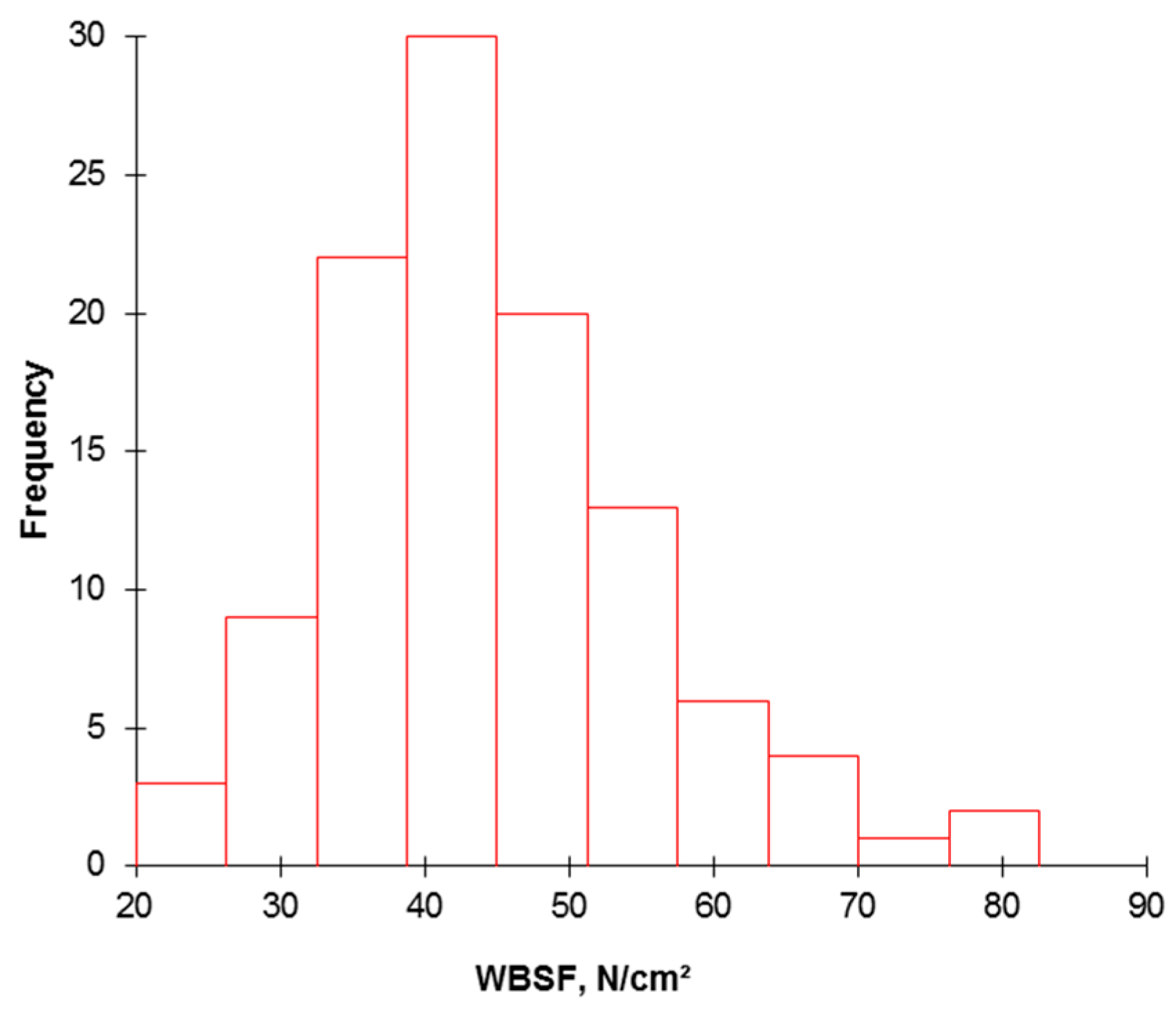
The descriptive analyses of the information (mean, SD, and minimum and maximum ranges) at each level of the continuum are given in Table 1, Table 2, Table 3 and Table 4. Warner-Bratzler shear strength (WBSF) is a routine instrumental measure out used as a proxy for sensory testing for meat tenderness. The WBSF values ranged from 23.55–81.49 N/cm², with an average of 44.6 N/cm² (SD 11.21 N/cm²). The coefficient of variation was, therefore, 25.1%. This indicates a high variability in tenderness of the population of PDO Maine-Anjou (Figure 2). This was reported past previous studies [26,27,28,29,30] and is a mutual result in the field of meat texture quality. Yet, there is scarcity in the studies bachelor on meat tenderness of PDO Maine-Anjou breed rather than this database to perform any comparisons.

The best WBSF PLS model retained 24 variables to explicate tenderness variability (Tabular array 5). From the whole 59 explanatory (contained) variables included in the PLS model, 35 had variable importance in the projection (VIP < 0.80) and were removed based on the filter method (Figure one). This footstep improved the variation explained in the second model (R^twoX: from 0.17–0.31) and the powerful of the link (R²Y: from 0.37–0.64) with the dependent variable that is WBSF. The concluding model explained 75% of the variability of WBSF (Tabular array 5). Amongst the 24 variables, six were from farm level (age of weaning; grass diet, %; haylage nutrition, %; nascence month; type of animal (meat or dairy) and physical action at farm, %), 4 from slaughterhouse level (color and tenderness scores of the carcasses; ribeye weight and EUROP conformation score), 11 were from the muscle level and mostly they were tenderness protein biomarkers (fiber area, µ-calpain, m-calpain, SOD1, ICDH, DJ-1, PGM1, HSP70-8, LDH, and total and insoluble collagen) and three were from meat level (pHu, redness (a*) and yellowness (b*)). The ranks of each of the 24 variables in the model based on their VIP are further given in Table v.

The objective with respect to implementing decision tools is to propose a model that accurately explains beef tenderness by learning elementary decision rules inferred from the private values of WBSF using the retained potential predictors from Table 5. Accordingly, the best determination tree congenital using the retained variables in the PLS model was that of CHAID method (Figure 3). CHAID is a recursive division based on the χ²-test, which is used to select the best split at each step [31]. Briefly, a CHAID tree is a decision tree that is built by repeatedly splitting subsets of the space into 2 or more child nodes, beginning with the first whole dataset [32]. To define the best split at any node of decision tree, whatsoever allowable pair of categories of the independent variables is merged until at that place is no statistically pregnant departure within the pair with respect to the target variable. CHAID has also the peculiarity to continue stepwise, thus being more proficient at treatment interactions betwixt explanatory variables, which are available from an examination of the tree. So, the final nodes of the tree identify subcategories adamant by unlike sets of explanatory variables. The WBSF CHAID conclusion tree in this trial (Effigy 3A) has 4 levels and 11 nodes out of which half-dozen are considered as last (they do not split farther). From the 6 concluding nodes, the tree immune identifying 3 different classes of WBSF (differing in their tenderness: Tender (2 nodes), Medium (1 node) and Tough (three nodes)) using five splitting variables only. The resultant model yielded an overall predictive accurateness of 69.iv% compared to the raw data of each individual ascertainment of WBSF.

From the five splitters, iii were the first drivers of the PLS model (highlighted in bold character in Tabular array v). The first splitter was full collagen and generated two groups. As expected, the 15 steaks of the showtime node (right of determination tree) with total collagen ≥ 3.vi μg OH-proline/mg had the highest WBSF values (mean value = 50.3 North/cm²) and considered as Tough meat [27,33]. After that, the 2nd group (northward = 95) was clustered past µ-calpain at a threshold of 169 AU. The group on the correct (n = 26) was and so separated by ultimate pH at a threshold of five.55 into 14 medium steaks (WBSF hateful value = 43.4 N/cmⁱⁱ) and 12 very tender steaks (WBSF mean value = 36.2 N/cm²). The grouping on the left (n = 69) was separated by the age of weaning of the animals into a final tough group (WBSF ≥ 45, n = 18) and a medium group of 51 steaks, which were then categorized past fiber area at a threshold of 3100 µm² into 30 tender (WBSF hateful value = 39.four N/cm²) and 21 tough steaks (WBSF mean value = 48.ane N/cm²). The mean values of WBSF among the three tenderness categories are 38.9 ± viii.1 Northward/cm^two, 43.iv ± 6.6 Northward/cmⁱⁱ and 49.4 ± 12.0 N/cm² for tender, medium and tough steaks, respectively. Therefore, the CHAID conclusion tree could simply and easily apply the bigotry dominion based on five splitters to identify these iii tenderness categories.

It seems from the whole data of the continuum based on the PLS model and CHAID conclusion tree that muscle characteristics (from the muscle level) namely total collagen content, µ-calpain and fiber expanse, are the main potential discriminators/predictors of tenderness of PDO Maine-Anjou (Figure 3B). Collagen is well known to exist associated with the background of meat toughness [34,35]. In a meta-analysis on the master parameters affecting collagen amount and its heat-solubility, Blanco et al. [36] hypothesized that total collagen content is different among muscles just with loftier amounts at birth, thereafter decreasing from birth to puberty as a part of muscle growth [35]. They farther linked their model to proteolysis, in line to the involvement of µ-calpain, cantankerous-sectional area of the fibers and age of weaning of the animate being. In a recent metadata of 308 young bulls that were categorized into three tenderness classes, full collagen was a discriminator of the built tenderness classes with a mean value for the tough class of three.51 µg OH-prol·mg⁻¹ DM. These findings concord with the negative link of collagen with tenderness evaluated by trained panelist or instrumental, as reported in numerous studies [13,14,17,37] and reviewed past Lepetit [38,39].

The two other variables are related to farm level (rearing practices) past historic period of weaning or at the meat level by ultimate pH. Accordingly, the determination tree (Effigy 3A) allowed to identify that a steak of the PDO Maine-Anjou was considered tender (lowest WBSF: < 40N/cm²) if it matched the following ii rules:

(i)

IF (total collagen < 3.half-dozen μg OH-proline/mg) AND (µ-calpain ≥ 169 AU) AND (ultimate pH < v.55) And then meat was very tender (hateful WBSF values = 36.two North/cm^two, n = 12); or

(ii)

IF (total collagen < 3.vi μg OH-proline/mg) AND (µ-calpain < 169 AU) AND (age of weaning < vii.75 months) AND (cobweb area < 3100 µm²) THEN meat was tender (mean WBSF values = 39.4 North/cm², due north = thirty).

In add-on to the predictive rules allowed by the statistical approach applied in this study, possible biological mechanisms behind meat tenderness determinism of PDO Maine-Anjou breed are further revealed. It seems that the concluding tenderness of this breed is mainly related to the extent breakup of structural properties in the muscle and to the background toughness related to connective tissue. This is in agreement with the contempo findings of a proteomic study based on a sub dataset of viii PDO Maine-Anjou cows categorized into four tender (WBSF < 31 N/cm²) and 4 tough (N > 60 N/cm²) samples [40]. In this written report, the authors identified eight potential biomarkers explaining differences in tenderness, of which six are structural proteins. The interesting links allowed by the conclusion tree inside pH drop presented by ultimate pH and proteolysis by the abundance of µ-calpain back up these findings. Furthermore, these are consequent with several studies from the large literature [41,42,43,44]. For example, an earlier work by Dransfield et al. [45] reported strong relationship between glycolysis and μ-calpain activity with a potent outcome on final tenderness of meat.

The involvement of age at weaning and the cross-sectional surface area of the fibers in the prediction of tenderness may be explained past 2 reasons. Showtime, it is known that animal growth touch muscle development and consequently its limerick including connective tissue [46], evaluated in this written report by collagen content and solubility. Second, animate being growth had important consequences on protein turnover know to influence the last qualities of meat [47]. Indeed, previous studies have reported pregnant relationships between the speed of development of the animal and therefore its carcass composition with tenderness of cows according to age at weaning [48]. Overall, these results allow us to advise the PLS—CHAID determination trees every bit an interesting tool for validation on other types of animals and other qualities of meat for utilise by the farmers every bit well equally the slaughterers in order to allocate (or predict) the potential quality of carcasses soon subsequently slaughter.

4. Conclusions

The purpose of this trial was to investigate the usefulness of combining chemometrics and auto learning tools to predict tenderness of PDO Maine-Anjou cows. Starting time, we analyzed the potential of Partial Least Squares to select the main variables (or variables of interest) from the continuum to explain WBSF of ribeye steaks. The filter method allowed retaining 24 variables from 59 to explain WBSF variability. Second, using the CHAID decision tree equally the best algorithm method amid others, the 110 steaks were categorized into three tenderness classes using five splitters: full collagen, µ-calpain, cobweb surface area, age of weaning and ultimate pH. Three of these potential predictors belong mainly to the muscle level and the two terminal other predictors to the farm and meat levels. The original statistical approach applied in this trial allowed us to properly group steaks for their tenderness potential using variables of the farm-to-meat continuum data. In the hereafter, this proposed approach would be combined with sensory scores of tenderness (using trained panelists or consumers) to better the prediction power and accuracy equally well the validation of the retained splitters equally predictors of PDO Maine-Anjou tenderness. Finally, the proposed tool would be further adopted for validation on other fauna types and volition exist proposed for use past the beef sector to accurately categorize carcasses according to their tenderness potential. This would be benign at both the economical and consumer levels.

Author Contributions

Conceptualization, M.G., 5.M., Southward.C. and B.P.; methodology, Thousand.1000., V.M. and B.P.; validation, V.M. and B.P.; formal assay, Grand.Thou.; investigation, S.C. and K.Chiliad.; resources, V.M., S.C. and B.P.; data curation, G.Yard., S.C., and B.P.; writing—original typhoon preparation, M.Yard.; writing—review and editing, V.1000., S.C. and B.P.; visualization, M.G.; funding acquisition, V.M., S.C. and B.P.

Funding

This research was funded by the INRA and Pays de la Loire Region (PSDR grant PA−PEss-AOCMA_2009). The grant of project S3-23000846 given to M.One thousand was funded by Région Auvergne-Rhône-Alpes and Fonds Européens de Développement Régional (FEDER).

Acknowledgments

Authors thank the PDO Maine-Anjou association, ADEMA and the Elivia slaughterhouse for their assist in the surveys, the farm selection and the sample drove. The authors thank the many colleagues involved in this project, namely, Alberic Valais, Guillain Le Bec and Ghislain Aminot from SICA Rouge des Preés and Didier Micol from INRA for their assistance in data collection, the direction and slaughter of animals, muscle sampling, and biochemical measurements. The authors convey special thanks to Nicole Dunoyer and Jeremy Huant for their technical help concerning the biomarkers quantifications past Dot-Blot and David Chadeyron for myosin heavy bondage quantification past electrophoresis.

Conflicts of Interest

The authors declare no conflict of interest.

References

1. Miller, 1000.F.; Carr, Thousand.A.; Ramsey, C.B.; Crockett, G.L.; Hoover, L.C. Consumer thresholds for establishing the value of beef tenderness. J. Anim. Sci. 2001, 79, 3062–3068. [Google Scholar] [CrossRef] [PubMed]
2. Henchion, Chiliad.; McCarthy, M.; Resconi, Five.C.; Troy, D. Meat Consumption: Trends and Quality Matters. Meat Sci. 2014, 98, 561–568. [Google Scholar] [CrossRef] [PubMed]
3. Troy, D.J.; Kerry, J.P. Consumer perception and the role of science in the meat industry. Meat Sci. 2010, 86, 214–226. [Google Scholar] [CrossRef] [PubMed]
4. McCarthy, Due south.Northward.; Henchion, M.; White, A.; Brandon, K.; Allen, P. Evaluation of beef eating quality by Irish gaelic consumers. Meat Sci. 2017, 132, 118–124. [Google Scholar] [CrossRef] [PubMed]
5. Ferguson, D.Chiliad.; Bruce, H.L.; Thompson, J.K.; Egan, A.F.; Perry, D.; Shorthose, W.R. Factors affecting beef palatability - farmgate to chilled carcass. Aust. J. Exp. Agric. 2001, 41, 879–891. [Google Scholar] [CrossRef]
6. Gagaoua, M.; Monteils, 5.; Picard, B. Information from the farmgate-to-meat continuum including omics-based biomarkers to better understand the variability of beef tenderness: An integromics approach. J. Agric. Food Chem 2018, 66, 13552–13563. [Google Scholar] [CrossRef] [PubMed]
7. Gagaoua, M.; Picard, B.; Monteils, 5. Associations amongst animal, carcass, muscle characteristics, and fresh meat color traits in Charolais cattle. Meat Sci. 2018, 140, 145–156. [Google Scholar] [CrossRef] [PubMed]
8. Gagaoua, M.; Picard, B.; Monteils, Five. Cess of cattle inter-individual cluster variability: The potential of continuum data from the farm-to-fork for ultimate beef tenderness direction. J. Sci Food Agric. 2019, 99, 4129–4141. [Google Scholar] [CrossRef]
9. Gagaoua, M.; Picard, B.; Soulat, J.; Monteils, V. Clustering of sensory eating qualities of beef: Consistencies and differences inside carcass, muscle, beast characteristics and rearing factors. Livest. Sci. 2018, 214, 245–258. [Google Scholar] [CrossRef]
10. Gagaoua, Thousand.; Picard, B.; Monteils, V. Beef quality management based on the continuum information from farmgate-to-meat: Which statistical strategies for meat science metadata analyses? In Proceedings of 24. Rencontres autour des recherches Ruminants (3R), Paris, France, 5–half-dozen December 2018; pp. one–5. [Google Scholar]
11. Gagaoua, M.; Monteils, V.; Couvreur, S.; Picard, B. Identification of Biomarkers Associated with the Rearing Practices, Carcass Characteristics, and Beef Quality: An Integrative Approach. J. Agric. Nutrient Chem. 2017, 65, 8264–8278. [Google Scholar] [CrossRef]
12. Couvreur, S.; Le Bec, G.; Micol, D.; Picard, B. Relationships Between Cull Beefiness Cow Characteristics, Finishing Practices and Meat Quality Traits of Longissimus thoracis and Rectus abdominis. Foods 2019, 8, 141. [Google Scholar] [CrossRef] [PubMed]
13. Jurie, C.; Picard, B.; Hocquette, J.F.; Dransfield, E.; Micol, D.; Listrat, A. Muscle and meat quality characteristics of Holstein and Salers cull cows. Meat Sci. 2007, 77, 459–466. [Google Scholar] [CrossRef] [PubMed]
14. Gagaoua, M.; Terlouw, E.Thou.C.; Micol, D.; Hocquette, J.F.; Moloney, A.P.; Nuernberg, K.; Bauchart, D.; Boudjellal, A.; Scollan, Due north.D.; Richardson, R.I.; et al. Sensory quality of meat from eight different types of cattle in relation with their biochemical characteristics. J. Integr. Agric. 2016, fifteen, 1550–1563. [Google Scholar] [CrossRef]
15. Picard, B.; Barboiron, C.; Chadeyron, D.; Jurie, C. Protocol for high-resolution electrophoresis separation of myosin heavy chain isoforms in bovine skeletal muscle. Electrophoresis 2011, 32, 1804–1806. [Google Scholar] [CrossRef] [PubMed]
16. Gagaoua, M.; Terlouw, Eastward.K.C.; Picard, B. The study of protein biomarkers to understand the biochemical processes underlying beefiness colour evolution in immature bulls. Meat Sci. 2017, 134, 18–27. [Google Scholar] [CrossRef]
17. Dubost, A.; Micol, D.; Meunier, B.; Lethias, C.; Listrat, A. Relationships between structural characteristics of bovine intramuscular connective tissue assessed by image analysis and collagen and proteoglycan content. Meat Sci. 2013, 93, 378–386. [Google Scholar] [CrossRef] [PubMed]
18. Guillemin, North.; Meunier, B.; Jurie, C.; Cassar-Malek, I.; Hocquette, J.F.; Leveziel, H.; Picard, B. Validation of a Dot-Absorb quantitative technique for large scale assay of beef tenderness biomarkers. J. Physiol Pharm. 2009, 60 (Suppl. 3), 91–97. [Google Scholar]
19. Folch, J.; Lees, Grand.; Sloane Stanley, Thou.H. A unproblematic method for the isolation and purification of total lipides from animal tissues. J. Biol. Chem. 1957, 226, 497–509. [Google Scholar]
20. Lepetit, J.; Culioli, J. Mechanical properties of meat. Meat Sci. 1994, 36, 203–237. [Google Scholar] [CrossRef]
21. Gagaoua, One thousand.; Terlouw, C.; Richardson, I.; Hocquette, J.F.; Picard, B. The associations between proteomic biomarkers and beef tenderness depend on the end-point cooking temperature, the country origin of the panelists and breed. Meat Sci. 2019, 157, 107871. [Google Scholar] [CrossRef]
22. Picard, B.; Gagaoua, M.; Al Jammas, M.; Bonnet, M. Beef tenderness and intramuscular fat proteomic biomarkers: Consequence of gender and rearing practices. J. Proteom. 2019, 200, i–10. [Google Scholar] [CrossRef] [PubMed]
23. Mehmood, T.; Liland, Chiliad.H.; Snipen, L.; Sæbø, S. A review of variable selection methods in Partial Least Squares Regression. Chemom. Intell. Lab. Syst. 2012, 118, 62–69. [Google Scholar] [CrossRef]
24. Chong, I.-G.; Jun, C.-H. Performance of some variable selection methods when multicollinearity is nowadays. Chemom. Intell. Lab. Syst. 2005, 78, 103–112. [Google Scholar] [CrossRef]
25. Gagaoua, M.; Monteils, Five.; Picard, B. Decision tree, a learning tool for the prediction of beef tenderness using rearing factors and carcass characteristics. J. Sci. Food Agric. 2019, 99, 1275–1283. [Google Scholar] [CrossRef] [PubMed]
26. Belew, J.B.; Brooks, J.C.; McKenna, D.R.; Savell, J.W. Warner–Bratzler shear evaluations of 40 bovine muscles. Meat Sci. 2003, 64, 507–512. [Google Scholar] [CrossRef]
27. Shackelford, S.D.; Morgan, J.B.; Cross, H.R.; Savell, J.W. Identification of Threshold Levels for Warner-Bratzler Shear Force in Beef Peak Loin Steaks. J. Muscle Foods 1991, 2, 289–296. [Google Scholar] [CrossRef]
28. Wheeler, T.L.; Shackelford, Southward.D.; Koohmaraie, M. Sampling, cooking, and coring furnishings on Warner-Bratzler shear force values in beef2. J. Anim. Sci. 1996, 74, 1553–1562. [Google Scholar] [CrossRef]
29. Magnabosco, C.U.; Lopes, F.B.; Fragoso, R.R.; Eifert, Eastward.C.; Valente, B.D.; Rosa, Thousand.J.One thousand.; Sainz, R.D. Accurateness of genomic breeding values for meat tenderness in Polled Nellore cattle1. J. Anim. Sci. 2016, 94, 2752–2760. [Google Scholar] [CrossRef] [PubMed]
30. Jerez-Timaure, N.; Huerta-Leidenz, North.; Ortega, J.; Rodas-González, A. Prediction equations for Warner–Bratzler shear force using chief component regression analysis in Brahman-influenced Venezuelan cattle. Meat Sci. 2013, 93, 771–775. [Google Scholar] [CrossRef]
31. Kass, G.5. An Exploratory Technique for Investigating Large Quantities of Categorical Information. J. R. Stat. Soc. Ser. C (Appl. Stat.) 1980, 29, 119–127. [Google Scholar] [CrossRef]
32. Ture, Yard.; Tokatli, F.; Kurt, I. Using Kaplan–Meier analysis together with decision tree methods (C&RT, CHAID, QUEST, C4.5 and ID3) in determining recurrence-free survival of breast cancer patients. Expert Syst. Appl. 2009, 36, 2017–2026. [Google Scholar] [CrossRef]
33. Nian, Y.; Zhao, M.; O'Donnell, C.P.; Downey, One thousand.; Kerry, J.P.; Allen, P. Assessment of physico-chemic traits related to eating quality of immature dairy bull beef at unlike ageing times using Raman spectroscopy and chemometrics. Food Res. Int. 2017, 99, 778–789. [Google Scholar] [CrossRef] [PubMed]
34. Purslow, P.P. New developments on the role of intramuscular connective tissue in meat toughness. Annu. Rev. Nutrient Sci. Technol. 2014, 5, 133–153. [Google Scholar] [CrossRef]
35. Purslow, P.P. Contribution of collagen and connective tissue to cooked meat toughness; some paradigms reviewed. Meat Sci. 2018, 144, 127–134. [Google Scholar] [CrossRef] [PubMed]
36. Blanco, M.; Jurie, C.; Micol, D.; Agabriel, J.; Picard, B.; Garcia-Launay, F. Impact of animal and management factors on collagen characteristics in beefiness: A meta-analysis approach. Animal 2013, vii, 1208–1218. [Google Scholar] [CrossRef] [PubMed]
37. Dransfield, E.; Martin, J.-F.; Bauchart, D.; Abouelkaram, S.; Lepetit, J.; Culioli, J.; Jurie, C.; Picard, B. Meat quality and composition of three muscles from French cull cows and immature bulls. Anim. Sci. 2003, 76, 387–399. [Google Scholar] [CrossRef]
38. Lepetit, J. A theoretical approach of the relationships between collagen content, collagen cross-links and meat tenderness. Meat Sci. 2007, 76, 147–159. [Google Scholar] [CrossRef] [PubMed]
39. Lepetit, J. Collagen contribution to meat toughness: Theoretical aspects. Meat Sci. 2008, 80, 960–967. [Google Scholar] [CrossRef]
40. Beldarrain, Fifty.R.; Aldai, Northward.; Picard, B.; Sentandreu, E.; Navarro, J.L.; Sentandreu, M.A. Use of liquid isoelectric focusing (OFFGEL) on the discovery of meat tenderness biomarkers. J. Proteom. 2018, 183, 25–33. [Google Scholar] [CrossRef]
41. Gagaoua, M.; Terlouw, Eastward.1000.; Micol, D.; Boudjellal, A.; Hocquette, J.F.; Picard, B. Understanding Early Post-Mortem Biochemical Processes Underlying Meat Color and pH Reject in the Longissimus thoracis Muscle of Immature Blond d'Aquitaine Bulls Using Protein Biomarkers. J. Agric. Food Chem. 2015, 63, 6799–6809. [Google Scholar] [CrossRef]
42. Kendall, T.Fifty.; Koohmaraie, Yard.; Arbona, J.R.; Williams, S.E.; Young, L.L. Outcome of pH and ionic forcefulness on bovine thou-calpain and calpastatin activity. J. Anim. Sci. 1993, 71, 96–104. [Google Scholar] [CrossRef] [PubMed]
43. Hwang, I.H.; Thompson, J.1000. The interaction between pH and temperature decline early postmortem on the calpain system and objective tenderness in electrically stimulated beefiness Longissimus dorsi muscle. Meat Sci. 2001, 58, 167–174. [Google Scholar] [CrossRef]
44. Ouali, A.; Gagaoua, Yard.; Boudida, Y.; Becila, Southward.; Boudjellal, A.; Herrera-Mendez, C.H.; Sentandreu, Thousand.A. Biomarkers of meat tenderness: Present knowledge and perspectives in regards to our current understanding of the mechanisms involved. Meat Sci. 2013, 95, 854–870. [Google Scholar] [CrossRef] [PubMed]
45. Dransfield, E.; Etherington, D.J.; Taylor, M.A.J. Modelling post-mortem tenderisation—II: Enzyme changes during storage of electrically stimulated and non-stimulated beef. Meat Sci. 1992, 31, 75–84. [Google Scholar] [CrossRef]
46. Listrat, A.; Gagaoua, M.; Picard, B. Study of the Chronology of Expression of 10 Extracellular Matrix Molecules during the Myogenesis in Cattle to Meliorate Empathize Sensory Properties of Meat. Foods 2019, viii, 97. [Google Scholar] [CrossRef] [PubMed]
47. Moloney, A.P.; McGee, Grand. Factors Influencing the Growth of Meat Animals. In Lawrie's Meat Science, Viii Edition; Toldrá, F., Ed.; Woodhead Publishing: Sawston, Britain, 2017; pp. 19–47. [Google Scholar]
48. Meyer, D.50.; Kerley, One thousand.Southward.; Walker, E.Fifty.; Keisler, D.H.; Pierce, V.Fifty.; Schmidt, T.B.; Stahl, C.A.; Linville, One thousand.50.; Berg, E.P. Growth rate, trunk composition, and meat tenderness in early vs. traditionally weaned beefiness calves1,2. J. Anim. Sci. 2005, 83, 2752–2761. [Google Scholar] [CrossRef] [PubMed]

Effigy 1. Summary of the statistical arroyo highlighting the four principal statistical steps followed in this study for the selection of best variables from the 59-continuum data from subcontract-to-meat and and so Warner-Bratzler Shear force (WBSF) prediction/categorization into dissimilar classes using 3 decision tree algorithms to select the all-time method.

Figure one. Summary of the statistical approach highlighting the four main statistical steps followed in this study for the pick of all-time variables from the 59-continuum data from farm-to-meat and then Warner-Bratzler Shear strength (WBSF) prediction/categorization into different classes using 3 conclusion tree algorithms to select the all-time method.

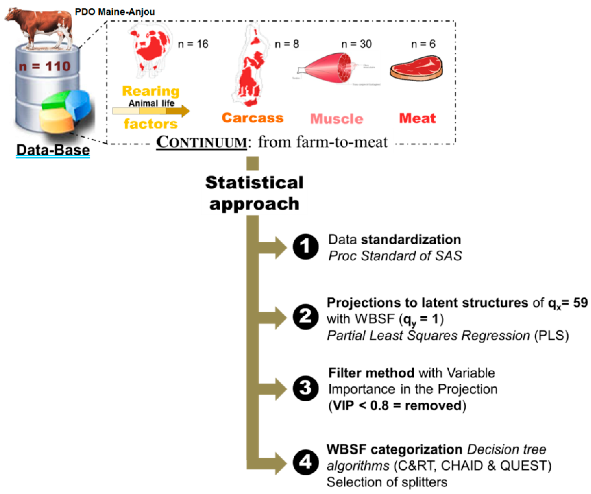
Figure 2. Histogram highlighting the relative frequency for meat tenderness assessed by WBSF on the 110 PDO Maine-Anjou cows.

Effigy 2. Histogram highlighting the relative frequency for meat tenderness assessed by WBSF on the 110 PDO Maine-Anjou cows.

Effigy 3. Categorization of the 110 steaks into different tenderness categories based on the decision tree. (A) Best decision tree obtained by the Chi-squared Automatic Interaction Detection (CHAID) method congenital using the listing of variables retained in Table 5 to predict correctly 69.4% of WBSF values into three tenderness categories (Red: Tough meat; Orange: Medium meat; Dark-green: Tender meat). The distribution of the animals in each WBSF cluster was used for accuracy measurement. At the get-go of the decision tree, all of the data (n = 110) are concentrated at a root node located at the top of the tree. This was so divided into two child nodes on the basis of an independent variable (1st splitter = total collagen), that creates the best homogeneity. The cutting-off value of each dividing splitter was calculated from the data of all the subjects. Therefore, the data in each kid node are more homogenous than those in the upper parent node. This process is continued repeatedly for each child node until all of the data in each node have the greatest possible homogeneity. This node is called a terminal node and no more than branches are possible. (B) Variance assay on the variables retained by the CHAID determination tree among the three WBSF (tenderness) categories that were all pregnant at p < 0.05 (Tukey'due south test). The mean values of WBSF amidst the 3 tenderness categories were further given at the bottom right of the graph B. Least-square means in the aforementioned graph with different superscript letters (a–c) are significantly different (p < 0.05).

Figure 3. Categorization of the 110 steaks into different tenderness categories based on the decision tree. (A) Best determination tree obtained past the Chi-squared Automatic Interaction Detection (CHAID) method built using the list of variables retained in Table five to predict correctly 69.iv% of WBSF values into 3 tenderness categories (Cherry: Tough meat; Orange: Medium meat; Green: Tender meat). The distribution of the animals in each WBSF cluster was used for accuracy measurement. At the beginning of the decision tree, all of the data (due north = 110) are concentrated at a root node located at the top of the tree. This was then divided into two child nodes on the basis of an independent variable (1st splitter = full collagen), that creates the best homogeneity. The cutting-off value of each dividing splitter was calculated from the data of all the subjects. Therefore, the data in each child node are more homogenous than those in the upper parent node. This process is connected repeatedly for each child node until all of the data in each node have the greatest possible homogeneity. This node is called a terminal node and no more branches are possible. (B) Variance analysis on the variables retained by the CHAID decision tree among the iii WBSF (tenderness) categories that were all significant at p < 0.05 (Tukey's examination). The hateful values of WBSF among the three tenderness categories were further given at the bottom right of the graph B. Least-foursquare means in the aforementioned graph with different superscript letters (a–c) are significantly different (p < 0.05).

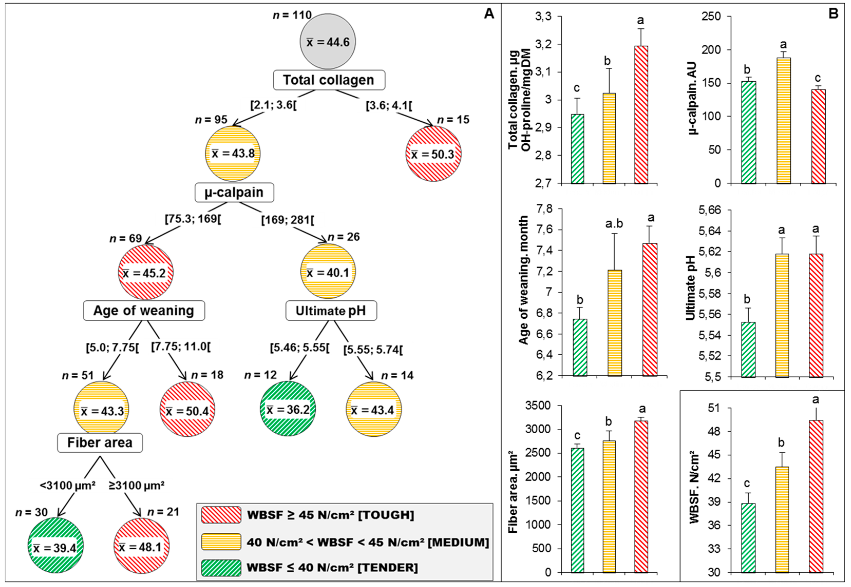
Table 1. Boilerplate values and variations of the data from the farm level describing the xvi variables of beast characteristics and finishing period ¹.

Table i. Average values and variations of the data from the farm level describing the 16 variables of animal characteristics and finishing catamenia ¹.

Variables	north	Mean	SD	Min	Max
Nascency weight (kg)	100	49.ix	4.91	38	66
Month of birth (ane–12)	110	-	-	ane	12
Genetic type (0: Beef or 1: Dairy)	110	-	-	0	one
Age of weaning (month)	107	7.2	one.07	five	11
Weaning duration 2	110	8.7	nine.41	0	36
Age at first calving (month)	110	32.4	4.09	18	43
Number of calving	110	3	2.05	1	ix
Suckling score (0–ten)	103	five.9	1.36	iii	9
Fattening elapsing (day)	110	98.half dozen	29.96	37	203
Haylage nutrition (%)	110	27.eight	36.98	0	100
Hay diet (%)	110	48.2	37.39	0	100
Grass diet (%)	110	24	32.ane	0	100
Daily concentrate diet (kg)	110	7.7	2.13	2	thirteen
Global concentrate diet (kg)	110	738	244	178	1330
Activity (%)	110	54	46.21	0	100
Age at slaughter (calendar month)	110	67.5	24.79	34	120

Table 2. Average values and variations of the data from the slaughterhouse level describing the 8 carcass characteristics.

Table ii. Average values and variations of the data from the slaughterhouse level describing the eight carcass characteristics.

Variables	n	Mean	SD	Min	Max
Carcass weight (kg)	110	438.ii	36.09	380	553
Conformation score (1–15 calibration) one	107	7.8	0.82	vi	10
5th rib weight (g)	110	3079	638	1793	5640
Muscle carcass weight (chiliad) ii	110	1882	403	1145	3478
Fat carcass weight (g) two	110	582	190	216	1338
Fat-to-muscle ratio in the fifth rib (% due west/west)	110	31.iii	10.17	16	85
Color score of the carcass (1–5) 3	105	2.9	0.38	2	iv
Tenderness score of the carcass (1–five) iv	105	3.4	0.65	ii	v

Tabular array three. Average values and variations of the data from the muscle level describing the xxx quantified characteristics in Longissimus thoracis muscle including protein biomarkers for the 110 cows.

Tabular array 3. Average values and variations of the information from the muscle level describing the 30 quantified characteristics in Longissimus thoracis muscle including protein biomarkers for the 110 cows.

Variables	Hateful	SD	Min	Max
a. Contractile properties by myosin fibers label
Cobweb area. µmtwo	2906	646	1762	5203
MyHC-I, %	31.2	7.37	15.22	69
MyHC-IIa, %	56.half dozen	12.78	23.76	84.78
MyHC-IIx/b, %	12.2	xiv.03	0	53.91
b. Metabolic properties by metabolic enzyme activities
LDH (μmol·min−1·g−one)	i.05	0.33	0.31	2.26
ICDH (μmol·min−1·g−one)	703	109	491	939
c. Intramuscular connective tissue properties
Full collagen μg OH-prol·mg−1 DM	iii.1	0.42	2.08	4.06
Insoluble collagen μg OH-prol·mg−1 DM	2.4	0.33	1.61	3.26
Soluble collagen %	twenty.eight	ii.94	14.85	26.58
d. Poly peptide biomarkers quantified past Dot-Blot (in arbitrary units)
Heat stupor proteins
CRYAB	226.4	83.96	59.04	576.89
Hsp20	164.8	45.45	59.84	306.74
Hsp27	79.7	19.83	36.88	134.56
Hsp40	130.5	20.97	96.09	280.56
Hsp70-1A	111.four	24.81	61.29	180.36
Hsp70-1B	120.i	26.16	seventy.38	187.36
Hsp70-viii	184.5	49.43	50.12	432.19
Hsp70-Grp75	144.v	thirty.5	87.12	213.24
Metabolism
Enolase 3 (ENO3)	144.iii	36.22	78.74	258.12
Phosphoglucomutase i (PGM1)	101	27.26	46.88	254.36
Structure
α-Actin	122.7	40.37	56.99	266.fourteen
Myosin binding protein H (MyBP-H)	90.two	27.49	42.05	184.32
Myosin calorie-free chain 1F (MyLC-1F)	63.8	12.91	33.23	91.06
Mysoin heavy concatenation IIx (MyHC-IIx)	124.9	xviii.55	eighty.91	182.28
Oxidative stress
Superoxide dismutase [Cu-Zn] (SOD1)	101.5	37.92	23.95	167.44
Peroxiredoxin 6 (PRDX6)	106.2	17.41	73.78	163.74
Protein deglycase (DJ1)	ninety.six	13.9	58.12	146.92
Proteolysis
µ-calpain	151.7	38.24	75.28	281.08
chiliad-calpain	96.1	12.62	64.69	124.75
Apoptosis and signaling
Tumor protein p53 (TP53)	118.three	22.31	78.36	175.78
H2A Histone Family Member Ten (H2AFX)	98.vii	nineteen.01	58.72	153.83

Table 4. Descriptive statistics of the half-dozen variables from the meat level respective to meat quality traits measured in Longissimus thoracis muscle.

Table four. Descriptive statistics of the half dozen variables from the meat level respective to meat quality traits measured in Longissimus thoracis muscle.

Variables	n	Mean	SD	Min	Max
Warner-Bratzler shear force (North/cmtwo)	110	44.six	11.21	23.55	81.49
Intramuscular fat (IMF) content (% west/w)	110	sixteen.3	6.18	6.fifteen	40.34
Ultimate pH (pHu)	107	5.6	0.1	5.34	6.22
Lightness (L*)	110	39.vii	ii.iii	34.36	46.84
Redness (a*)	110	8.8	1.24	iv.17	11.77
Yellowness (b*)	110	7.4	1.43	4.02	11.42

Table v. Best Partial Least Squares (PLS) model of Warner-Bratzler Shear force (WBSF) showing the ranking of the 24 retained variables from the continuum data from farm-to-meat and their variable importance in the projection (VIP) values.

Tabular array 5. Best Partial Least Squares (PLS) model of Warner-Bratzler Shear force (WBSF) showing the ranking of the 24 retained variables from the continuum data from farm-to-meat and their variable importance in the projection (VIP) values.

Variables of the Continuum from Farm-To-Meat Data	Rank	VIP
Subcontract level: rearing factors and animal characteristics
Age of weaning, calendar month	three	1.99
Grass diet, %	ten	i.31
Haylage diet, %	14	1.12
Birth month	15	1.xi
Type of animal (meat or dairy)	xvi	0.97
Physical activity at farm, %	24	0.84
Slaughterhouse level: carcass characteristics
Color score, 1–v scale	v	1.8
Carcass tenderness score, i–5 calibration	21	0.9
Ribeye weight, grand	20	0.94
EUROP Conformation score, ane–15 calibration	23	0.87
Muscle level: protein biomarkers
Cobweb area, µmtwo	2	ii.01
SOD1, AU	4	1.94
thousand-calpain, AU	6	i.64
ICDH, μmol·min−1·thou−1	7	ane.57
Protein deglycase (DJ-i), AU	9	ane.51
PGM1, AU	11	1.27
Insoluble collagen, μg OH-proline/mg DM	xiii	one.18
HSP70-viii, AU	17	0.97
µ-calpain, AU	18	0.96
Total collagen, μg OH-proline/mg DM	nineteen	0.96
LDH, μmol·min−1·1000−1	22	0.89
Meat level: meat quality traits
pHu	i	3.29
Redness (a*)	eight	one.53
Yellowness (b*)	12	ane.27

© 2019 by the authors. Licensee MDPI, Basel, Switzerland. This article is an open access article distributed nether the terms and conditions of the Creative Eatables Attribution (CC Past) license (http://creativecommons.org/licenses/by/iv.0/).

We employ cookies on our website to ensure you lot get the best experience.
Read more about our cookies here.

Nosotros have just recently launched a new version of our website.
Assistance usa to further improve by taking part in this short v minute survey here. hither.

wadesumbeyouned.blogspot.com

Source: https://www.mdpi.com/2304-8158/8/7/274/htm

Share this post